At trade shows and on-site events, it is difficult to illustrate the benefits and functionality of data science and machine learning, especially when theory alone is not enough.
This gave rise to the idea of creating a physical prototype whose data would be analyzed live using machine learning methods. We decided to use an existing model and equip it with additional sensors.
Table of Contents
1. Data collection – construction of the sensor system
2. Architecture
3. (Sensor) data processing
4. Evaluation – anomaly detection
4. Types of anomaly detection
4. Distribution-based methods
4. Density-based methods
4. Anomaly detection vs. classification
4.5 Anomaly detection for the excavator use case
4.6 Transferring the excavator use case to reality
It already has 7 motors that move individual parts of the excavator and can be controlled via a smartphone app.
In this blog article, we describe how such a model can be equipped with additional sensors, what special features there are in the processing of sensor data, and how data mining methods can be used to implement real-time monitoring of the sensors (with outlier detection).
Data collection – Construction of the sensor system
The excavator's seven motors are controlled via "hubs." These establish a connection to the smartphone app via Bluetooth. To detect load situations, we measure the voltage applied to the motors. The voltage can be measured in parallel, so none of the existing connections had to be disconnected. Instead, thin wires were soldered to the contact points.
These wires conduct the voltage to a circuit board equipped with an ESP8266. The ESP8266 is a circuit board chip with a Wi-Fi module and can be programmed. The ESP8266 reads the applied voltages in less than a second.
Architecture
The readings are sent via Wi-Fi to an endpoint for data reception. This endpoint performs several actions:
- Puts the data in chronological order.
The ESP8266 does not have a clock and therefore cannot provide a timestamp for the sensor data. The IP protocol does not specify a strict order for data packets. This means that a later measurement may arrive before the previous measurement. To get around this problem, the ESP8266 sends an incrementing counter so that the measurements can be put in order based on this. - Stores the measurements in the database so that a history is available, which can be analyzed using machine learning and used to train models.
- Performs anomaly detection. In this particular case, we opted for outlier analysis (also known as anomaly detection). In order to use the results of this model, it must be applied to newly arriving data.
- Forward the data to the dashboard so that it can be viewed as quickly as possible and, if necessary, a user/operator can take action.
(Sensor) data processing
There are a few points to consider when collecting and evaluating data (especially for data scientists).
Sensor data usually comes in as a stream, i.e., a continuous flow of data, and is then stored with a timestamp and reference to the sensor. This ensures that it can be clearly assigned to the machine. However, other data such as master data, order, or maintenance information can often only be assigned using the combination of "machine and timestamp or time period." The time components play a rather subordinate role in "classic" systems—whether a malfunction occurred 10 minutes later or earlier, for example, is irrelevant when it comes to troubleshooting.
In contrast, thousands of sensor points can arrive in 10 minutes, which are then incorrectly classified as "malfunctions" or the opposite. This makes subsequent evaluation very difficult. This problem can be solved by including the sensors themselves. When a system has a malfunction, it usually stops working, and in many cases there is a sensor that indicates whether the machine is running or not. Accordingly, the time of the malfunction can be taken as an approximate value and an exact time stamp can be derived from the sensor values (using threshold values, for example).
Another problem with sensor data streams is that they should be evaluated over a period of time. Some sensors tend to fluctuate. This may be due to inaccuracies in the sensor. However, it may also be that the property being measured varies greatly in a natural way.
An example:
You have the engine speed from many car journeys and want to compare them in terms of wear and tear. Some drivers tend to drive at a leisurely pace at a constant speed, while others tend to accelerate sharply and then brake again. A human being would quickly recognize the resulting "spikes" in the sensor curves and assume that the wear and tear is higher in the second profile.
But how can this be evaluated using machine learning?
The average engine speed can then be identical for all journeys. And particularly high and low speeds can also be found in every profile, because forward-thinking drivers sometimes have to accelerate or brake. So if a model is applied to this data without preprocessing, it could, in the best case scenario, learn that high speeds lead to higher wear and tear. However, this only happens if the proportion of "sporty driving" is also high. Otherwise, this would be lost in the general population. Fortunately, there are a number of mathematical indicators that can describe sensor curves, i.e., sensor values over time. This makes what a human being sees "at first glance" also visible to machine learning algorithms.
Variances such as MAD (mean absolute deviation) and AAD (absolute average deviation) are examples of metrics that would differ significantly between "sporty driving" and "moderate driving." This mathematical description also makes it easy to compare journeys of different lengths.
In our use case, we implemented outlier detection and, due to the simplicity of the sensors, decided not to use such a metric.
Evaluation – anomaly detection
Anomaly detection is a data mining technique used to identify unusual data points or observations that differ significantly from the rest of the data. This method is used to detect credit card fraud, system malfunctions, and production disruptions, among other things. Another use case is the identification of outliers for data cleansing.
Types of anomaly detection
There are numerous methods for outlier detection. The most common classification of these is into supervised, unsupervised, and semi-supervised methods.
Supervised learning
Labeled training data is available for learning the model. This means that it is known which data in the training data set are anomalies.
Semi-supervised learning
In the semi-supervised method, a model is trained based on a training set without anomalies, and the probability that a data set originates from the learned model is determined.
Unsupervised learning
Unlabeled training data is available for learning the model. This means that it is not known which data points are outliers. These methods assume that most data points are not outliers.
Univariate vs. multivariate methods
In addition to the type of model determination, models can also be classified according to the type of data dimensionality. There are univariate methods that are applied to one-dimensional distributed data, as well as multivariate methods for multidimensional distributed data.
Distribution-based methods
Interquartile range
In the interquartile method, a range is defined around the median of the sample set. All observations outside this range are identified as outliers.
GESD (Generalized Extreme Studentized Deviate Test)
Hypothesis tests are performed using the following test statistics
where x_Strich represents the sample mean and sigma represents the standard deviation of the sample.
The null hypothesis is that there are no outliers in the data set. The alternative hypothesis is that there are up to r outliers. r tests are performed as long as the test statistic exceeds a critical value. After each test, the data point with the greatest distance from the arithmetic mean is removed from the data set as a detected outlier and the test statistic is recalculated.
Density-based methods
Dbscan
Dbscan is a clustering method that determines clusters based on density. A point is considered dense if at least MinPts points are located in an environment with a radius of ɛ around the point. Various metrics, such as the Euclidean metric, can be used to determine the distance between points.
The procedure distinguishes between three types of points. The first type of points are core points. These are points that are dense. The second type are dense-reachable points. These are points whose e-neighborhood contains fewer than MinPt points but which are reachable from a core object of the cluster. Reachable means that the distance between two points is less than e. The third type are outliers. These are points that are not dense-reachable from other points.
A cluster is characterized as follows: All points in the cluster are densely connected. Two points are described as densely connected if there is a point from which both points are densely reachable. If a point is densely reachable from any point in the cluster, then this point is part of the cluster. This method therefore identifies outliers as independent, non-dense clusters.
Isolation Forests
This method is based on binary decision trees. To train a decision tree, a feature is selected at random and a random split is performed based on a value of that feature.
The isolation forest is then created by combining all isolation trees, using the average of their results.
Each observation is compared to the isolation value in a node. The number of isolations is called the path length. The assumption is that outliers have shorter path lengths than normal observations.
The outlier score is then determined as follows
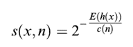
where h(x) is the path length of observation x, c(n) is the maximum path length of the tree, and n is the number of nodes in the tree. The value lies between 0 and 1. The higher the value, the more likely the observation is an outlier.
K-Nearest Neighbor
The K-Nearest Neighbor algorithm can also be used to identify anomalies. The distance of a data point to the k nearest neighbors is used as the measure for the outlier score.
Anomaly detection vs. classification
Classification is a supervised machine learning method for classifying data. It assumes that the individual labels occur with similar frequency.
Anomaly detection, on the other hand, assumes an imbalance between normal and abnormal data. There is a lot of normal data compared to a few anomalies. Furthermore, the training data does not necessarily have to be labeled, as described above.
Anomaly detection for the excavator use case
For the measured voltages, it was assumed that they could be considered independently of each other. In addition, only unlabeled data was available. Therefore, an unsupervised and univariate method must be used for anomaly detection.
The interquartile method has these characteristics and was therefore selected to perform anomaly detection. The results of the outlier detection are shown in the image below.
Transferring the excavator use case to reality
With this use case, we were able to show how sensor data can be monitored automatically. The anomaly was not particularly difficult to detect. However, such an algorithm can monitor many machines simultaneously non-stop and, if necessary, involve humans in the event of anomalies.
This is particularly interesting in the manufacturing industry. Faulty production can quickly lead to high levels of waste. Anomaly detection can also save time before intervention is required in this area.
Further use cases can be identified, particularly when additional data sources such as PM (Planned Maintenance) or QM (Quality Management) are included.
Using appropriate methods, data scientists can identify factors that influence wear and tear or quality, among other things. This information can then be used to positively influence these factors or monitor them closely.
Author: Bernd Themann
Kay Rohweder
Senior Manager
SAP Information Management
kay.rohweder@isr.de
+49 (0) 151 422 05 242


