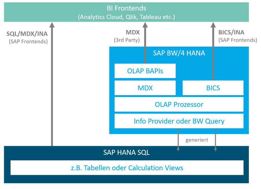
For a long time, SAP BW Query was the only option for providing data from SAP BW to BI front ends. With SAP HANA and the possibility of hybrid or mixed data models, a new option has been added: data can also be provided via SAP HANA Calculation Views.
In addition to modeling aspects, the two types of consumption also differ in the way data is provided. SAP BW queries are processed via the OLAP (Online Analytical Processing) processor and thus the ABAP server, whereas with HANA Calculation Views, this is handled by the database. Query and Calculation Views also communicate differently. The graphic below illustrates these relationships.
There are many reasons to choose one modeling variant over another. The decisive factor is which BI front end is to be used. In this blog post, we would like to limit ourselves to the differences in performance. We will focus on the query performance of the back end and will not compare the interfaces with each other (MDX, BICS, etc.).
Comparison based on scenarios
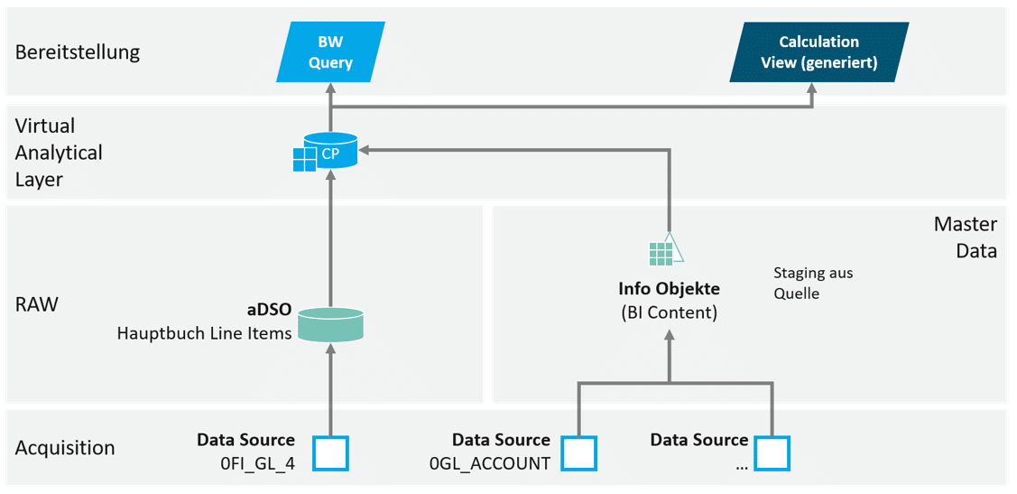
The performance comparison is based on the following data model. The data volume is approximately 34 million rows. The CompositeProvider provides 56 attributes and 4 key figures.
Performance is analyzed based on the following three use cases:
Detail level– Highly aggregated use case, additionally broken down by the characteristics "Fiscal year/period," "Document type," and "Valuation type."
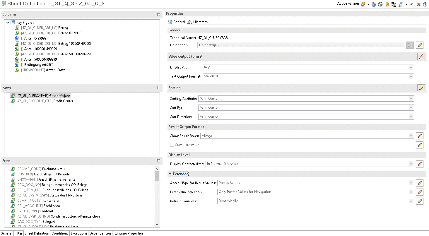
With logic– Highly aggregated use case, broken down by "fiscal year" and "profit center." In addition, restricted and calculated columns are used.
In detail: Practical measurement of execution times using BW query
The queries in the use cases considered below all have the same settings in the "General" and "Runtime Properties" tabs, which reflect the default configuration.
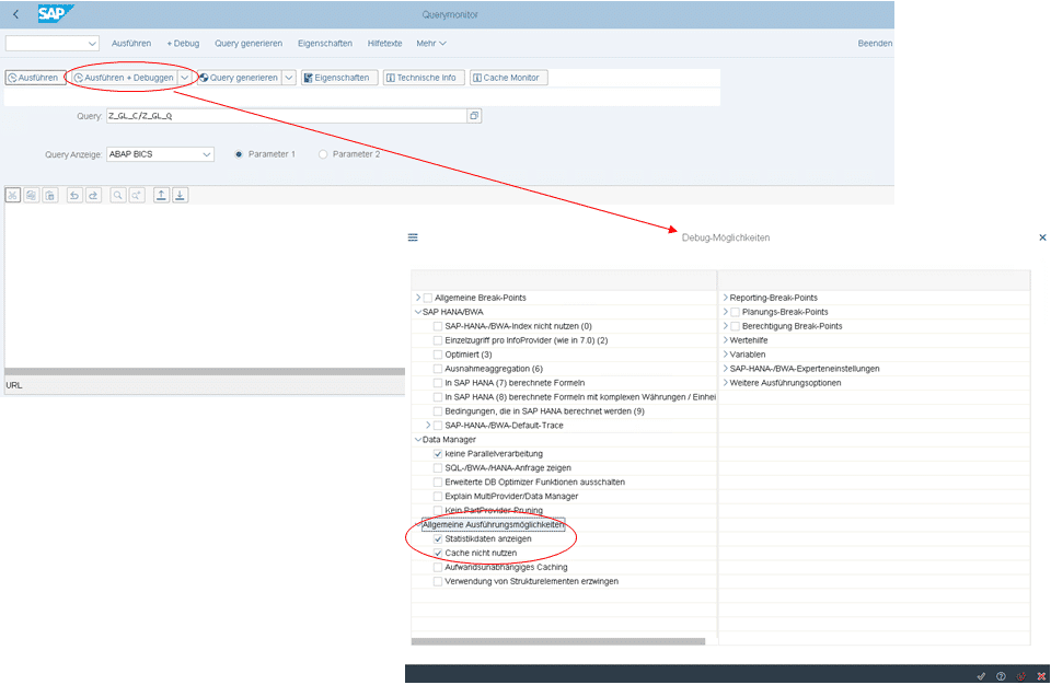
To analyze performance, the SAP transaction RSRT2 of BW/4HANA is used with the following settings. The execution is always performed three times and the average value is used as the rating.
To evaluate the statistics, it is important to know in advance that the analytic engine described in the introduction is used when queries are called up. Among other things, this consists of the sub-areas "Data Manager," which is responsible for reading the data, and "OLAP Services," which calculates and provides the query results.
Use case 01
Description
In the first scenario, the data basis is retrieved in a highly aggregated form. The query is broken down only by the four key figures, the fiscal year, and one additional characteristic (account type) that has up to five values. The remaining 54 characteristics are made available as free characteristics. Result rows are only output for the totals, i.e., only for the fiscal year characteristic. This rather narrow query returns a result set of 34 rows.
performance analysis
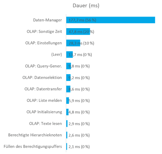
The following graphic shows the key events during the query call. The cumulative duration of each execution performed for testing purposes is shown in the highlighted area. This is used to determine the average execution time.
In this use case, the event "Data Manager," which belongs to the "Data Manager" subarea, has the greatest impact on the total time. This event measures the time as soon as it is called from the Analytic Engine. Other significant events belong to the OLAP Services subarea. These include "OLAP: Query Generation" (time measurement: checking the query definition and, if necessary, query generation), "OLAP Other Time" (runtimes not specified in detail, but within the Analytic Engine (OLAP)), and "OLAP: Settings" (time measurement: processing of interface settings and, in particular, announcement of the display hierarchy).
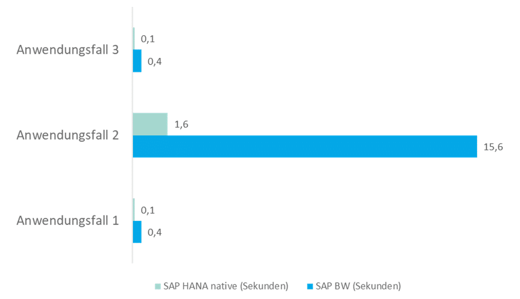
Result Average execution time: 0.4s
Use case 02
Description
Building on the first use case, this scenario outputs a higher number of rows. To do this, the breakdown is expanded to include the characteristics "Fiscal year/period," "Document type," and "Valuation type." This results in a result set of just under 94,000 rows.
Here, too, only result lines for the total amounts for the fiscal year are displayed.
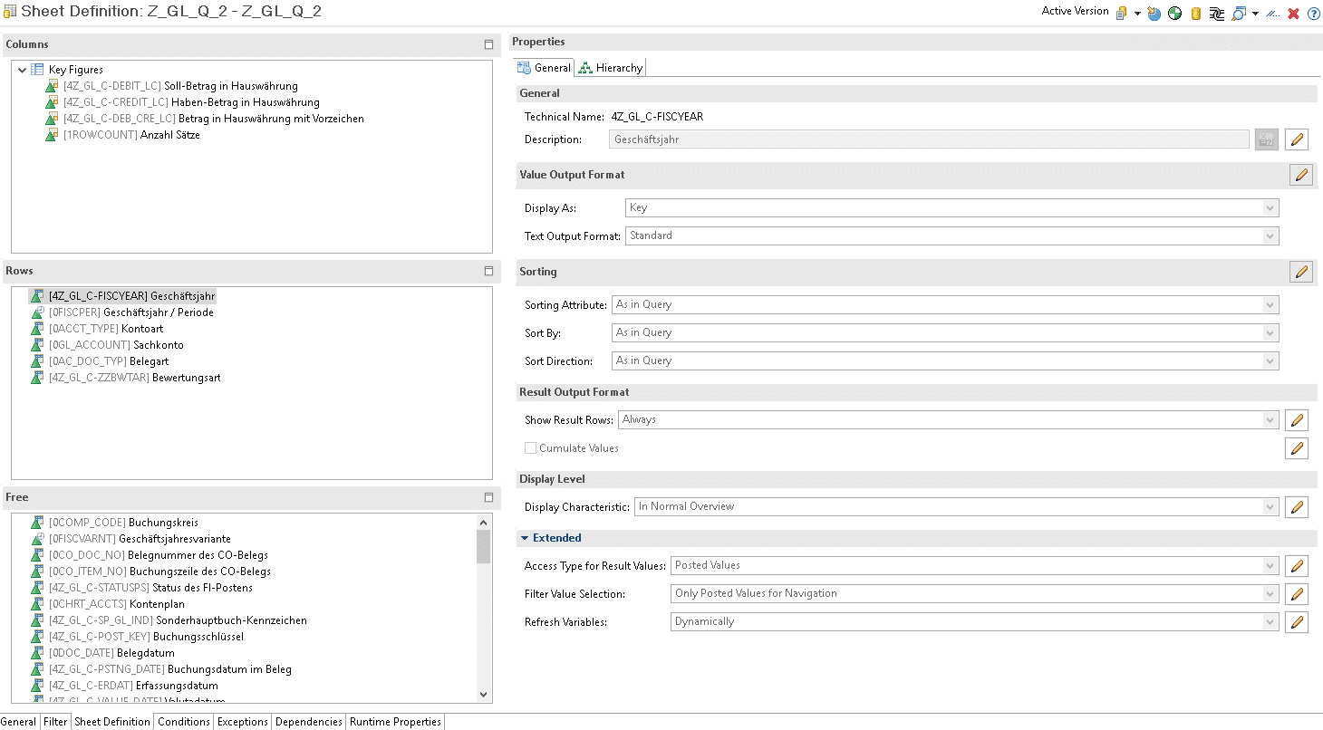
query definition
performance analysis
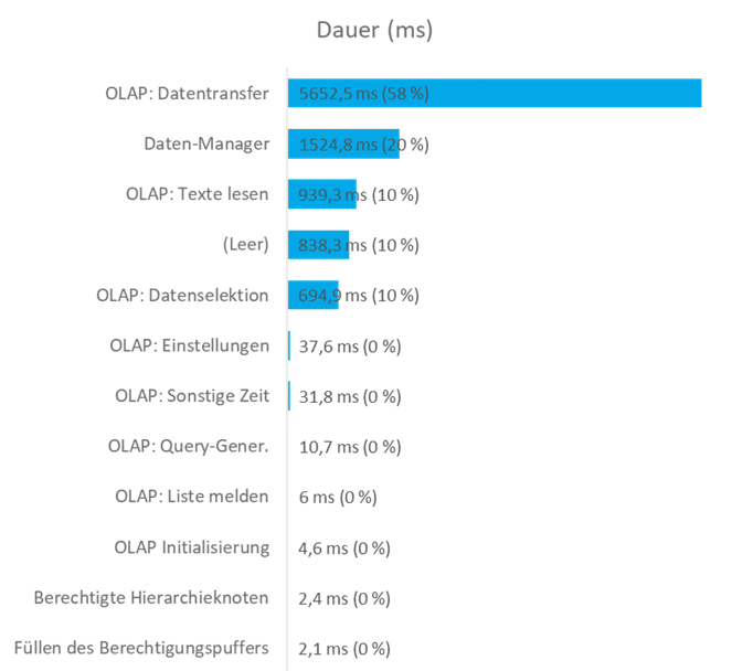
The following graphic shows the key events during the query call. The cumulative duration of each execution performed for testing purposes is shown in the highlighted area. This is used to determine the average execution time.
In this scenario, a large part of the execution time required falls within the "OLAP Services" subarea of the Analytic Engine. Of particular note here is "OLAP: Data Transfer," which transfers the data to the respective front end. This includes exception aggregations, currency conversions, formulas, decimal places, and the preparation of the result set based on the query definition. In addition, the events "OLAP: Data Selection" and "OLAP: Read Texts" also take up a considerable amount of time in this subarea. Other significant events can be assigned to the "Data Manager" subarea, and more specifically to the "Data Manager" event.
Result Average execution time: 15.6s!!!
Use case 03
Description
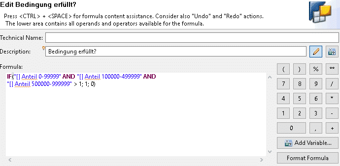
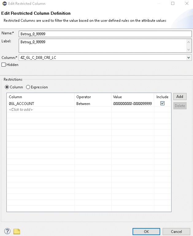
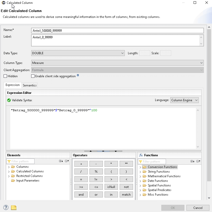
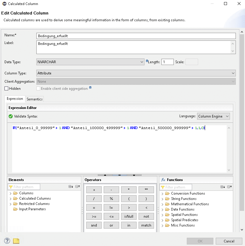
The third scenario again provides a relatively aggregated overview, broken down by fiscal year, profit center, and number of records. This is supplemented by restricted and calculated key figures, which are generated at runtime using logic. The additional key figures consist of:
Type
Description
Restricted key figures (simple)
Restricted by one characteristic each
Calculated key figures (simple)
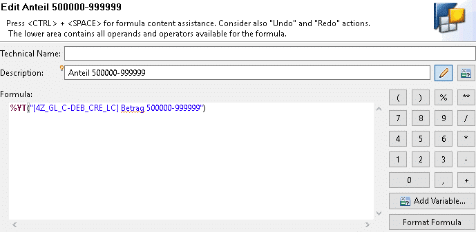
Example (see below)
Type
Description
More complex calculated key figure
Example (see below)
query definition
performance analysis
The following graphic shows the key events during the query call. The cumulative duration of each execution performed for testing purposes is shown in the highlighted area. This is used to determine the average execution time.
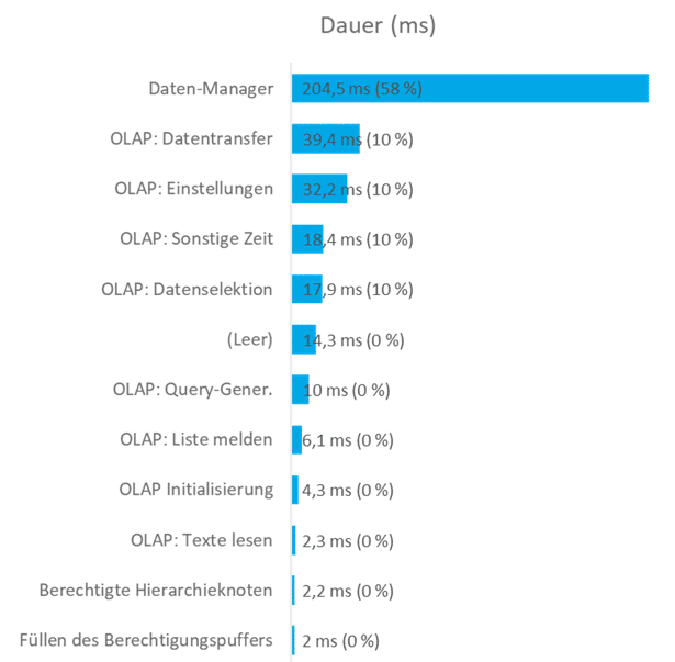
In this scenario, as in scenario 1, the Data Manager subarea tends to be more significant. Here, too, the "Data Manager" event accounts for almost half of the total execution time. In order of the most time-consuming events, this is followed by "OLAP: Data Transfer," "OLAP: Data Selection," and "OLAP: Settings."
Result Average execution time: 0.4s
In detail: Practical measurement of execution times using HANA CalculationView
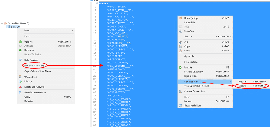
A HANA CalculationView is executed and processed on the SAP HANA database. The Plan Visualizer is used for performance analysis. For this purpose, a SELECT SQL statement is generated and executed in its entirety using the Plan Visualizer. Here, too, the average of three measurements is used to evaluate performance.
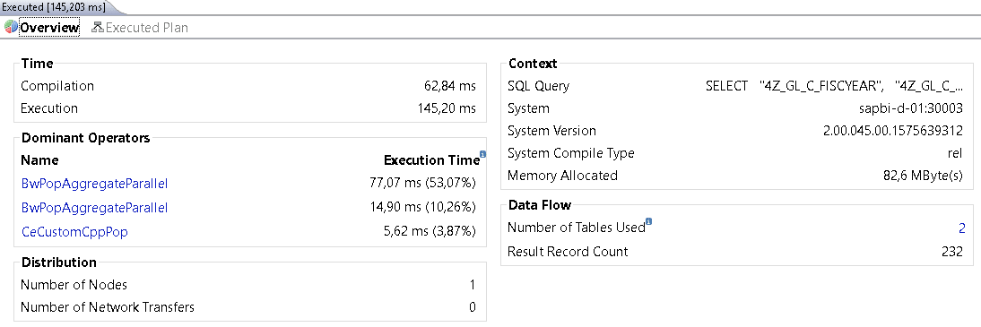
The following graphic provides an overview of the analysis results of the Plan Visualizer for executing a HANA CalculationView. Key performance indicators include the execution time ("Execution" in the "Time" section) and the memory (RAM) required for execution ("Memory Allocated" in the "Context" section). It is also very helpful to know how many tables are used and how large the result set is ("Number of Tables Used" and "Result Record Count" in the "Data Flow" section). Details about the operators used, the system, and the query itself are also provided.
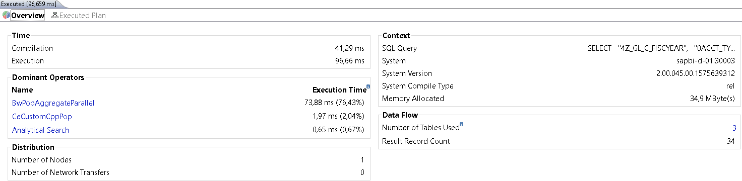
Use case 01
Description
The SAP BW query is replicated using the calculation view. This means that the data basis is highly aggregated and broken down according to four key figures, the fiscal year, and another characteristic (account type) that has up to five values.
Result rows are not output because this is not supported in Plan Visualizer.
performance analysis
The following illustration shows the result of one of the three designs using Plan Visualizer:
All dominant operators operate in the millisecond range, and memory consumption is lowest here compared to the other two scenarios.
Result Average execution time: 0.1s
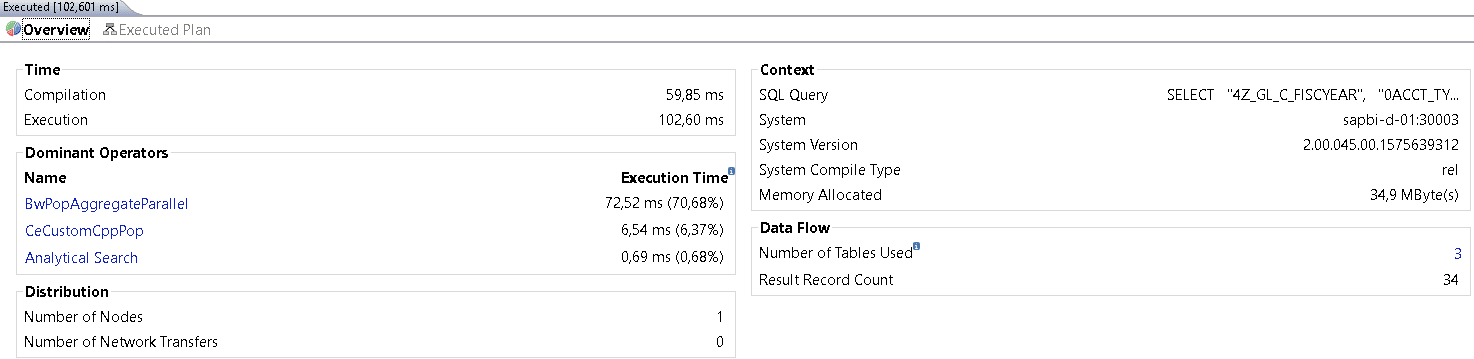
Use case 02
Description
Similar to the second use case with a BW query, a higher number of rows are output in this scenario. For this purpose, the breakdown is extended to include the characteristics "Fiscal year/period," "Document type," and "Valuation type." This results in a result set of just under 94,000 rows. Result rows are not output because this is not supported in Plan Visualizer.
performance analysis
The following illustration shows the result of one of the three designs using Plan Visualizer:
The dominant operators indicate that a rather time-consuming "column search" was apparently used in this case. The memory consumption of the three use cases tested is by far the highest here.
Result Average execution time: 1.6s
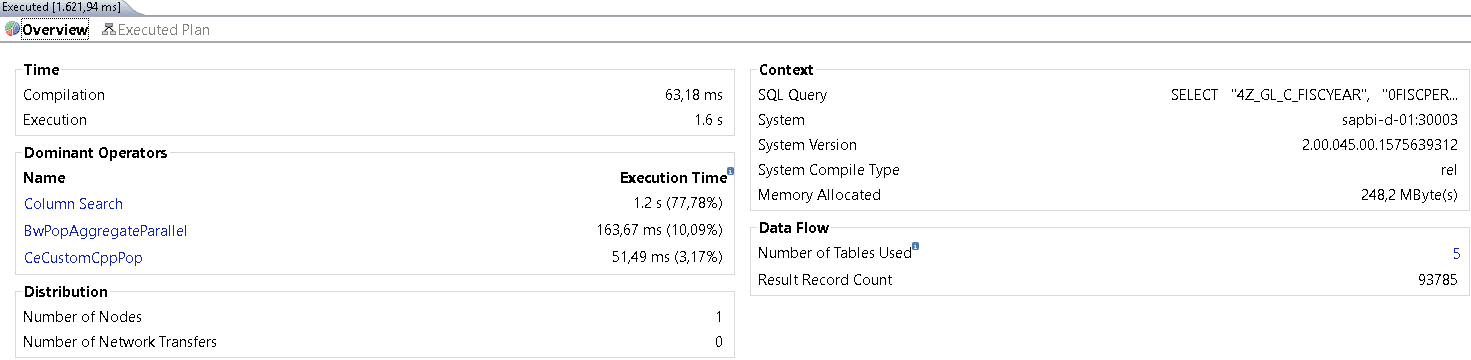
Use case 03
Description
As in use case 3, the third scenario uses a BW query to provide a relatively highly aggregated breakdown by fiscal year, profit center, and number of records. This is supplemented by restricted and calculated key figures, which are formed at runtime using logic. The additional key figures consist of:
Type
Description
Restricted key figures (simple)
Restricted by one characteristic each, example (see below)
Type
Description
Calculated key figures (simple)
Percentage function, example (see below)
Type
Description
More complex calculated key figure
IF query regarding the other three calculated key figures, example (see below)
performance analysis
The following illustration shows the result of one of the three designs using Plan Visualizer:
This use case also has execution times for the dominant operators in the millisecond range. In this case, however, memory is "only" in second place out of the three use cases.
Result Average execution time: 0.1s
Conclusion
Our analysis focused exclusively on the performance of both modeling types and does not represent a functional comparison. In this respect, our conclusion is limited to the performance of queries.
There is a clear winner here: the query speed of HANA Calculation Views is better than that of BW Query, especially when outputting large amounts of data. While the differences are almost negligible with smaller amounts of data, there is a clear difference when outputting the second use case. Compared to HANA CalculationView, BW Query and the OLAP processor lose too much time here because the data must first be transferred to the ABAP server before the query can be processed. This is reflected in the "OLAP: Data Transfer" event, which takes approximately 6 seconds * 2.
When it comes to performance, however, memory consumption is always important in addition to pure execution times. This should also be analyzed whenever possible. Although this blog post focused primarily on execution times, it can be noted that there were enormous differences in the memory required for the HANA CalculationViews (use case 1: ~35MB, use case 2: ~248MB, use case 3: ~82MB). These differences are certainly even more pronounced in more complex scenarios.
The results of the scenarios considered in this article are shown again graphically below. The graph clearly shows that HANA CalculationViews are faster than BW queries for the scenarios considered.
Since 1993, we have been operating as IT consultants for Data Analytics and Document Logistics, focusing on data management and process automation. We provide comprehensive support, from strategic IT consulting to specific implementations and solutions, all the way to IT operations, within the framework of holistic Enterprise Information Management (EIM). ISR is part of the CENIT EIM Group.