Historization of data with the ability to restore the historical status at any point in time, even retrospectively, is a core requirement for data warehouse systems.
In the case of SAP source systems, change records ("delta") are often already delivered to the Business Warehouse by SAP Business Content. However, non-SAP source systems often present a challenge to the Business Warehouse in that only a current status can be delivered, but not delta records with before/after images or timestamps ("Changed On" date).
Table of Contents
2. Alternative 2: Incremental historization of a full data source
2.1 Storage of change history in an ADSO
2.2 Creation of an ADSO "history" with the changes
2.3 Reporting on incremental history via calculation view
2.4 Rank function
2.6 Comparison of rank and aggregation function
3. Conclusion
For these cases, we will show here what options are available for a data warehouse in terms of historization and how these can be implemented in a modern (BW/4HANA) architecture using both BW and HANA tools.
Alternative 1: Snapshots
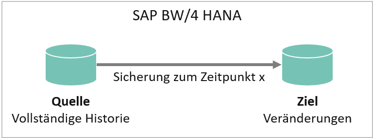
If a data source that is not delta-compatible is to be historized in order to report the data status on a selected key date, a regular full load with an additional key field (e.g., load date) may be the solution. However, with daily historization, this leads to an enormous increase in data volume, as a complete snapshot would have to be created every day.
Nevertheless, this approach is quite common and useful for monthly reporting, for example. Because complete "data slices" are recorded on a specific date, reporting is very simple and highly efficient, as only the relevant data slice needs to be filtered.
However, changes that have a lower granularity than the snapshot generation interval cannot be tracked or lead to the disproportionate bloating of the redundantly persistent data stock in the data mart mentioned at the beginning. An alternative to recording only the actual changes is therefore desirable.
Alternative 2: Incremental historization of a full data source
Storage of change history in an aDSO
If only a few records change each day, incremental historization may be the alternative. In this case, only changed, new, and deleted records are updated in the target InfoProvider with the new load date:
Incremental backup (changes only)
| Date (Key 1) | Key 2 | quantity | deletion flag | |
|---|---|---|---|---|
| 01.01.2020 | A | 10 | ||
| 01.01.2020 | B | 15 | ||
| 02.01.2020 | A | 20 | Change entry A | |
| 03.01.2020 | C | 5 | New entry C | |
| 04.01.2020 | B | 0 | X | Delete entry B |
Complete backup
| Date (Key 1) | Key 2 | quantity | |
|---|---|---|---|
| 01.01.2020 | A | 10 | |
| 01.01.2020 | B | 15 | |
| 02.01.2020 | A | 20 | Change entry A |
| 02.01.2020 | B | 15 | |
| 03.01.2020 | A | 20 | |
| 03.01.2020 | B | 15 | |
| 03.01.2020 | C | 5 | New entry C |
| 04.01.2020 | A | 20 | Delete entry B |
| 04.01.2020 | C | 5 |
Since only changed, deleted, or new records are updated in incremental historization, the amount of storage space required is significantly reduced. Reporting is still possible for each key date by using the current record of a key combination (see below → Reporting).
Creation of an "History" aDSO with the changes
There are various options for creating such an aDSO history.
If the DataSource of our source aDSO delivers a clean delta, we can simply process this further in our history aDSO. No problem. Even if a full transfer is made from the source, the change log from the source aDSO delivers a correct delta for the changes that have been made. With SAP BW/4 HANA, this function has been further enhanced by the identification of deletions (snapshot setting).
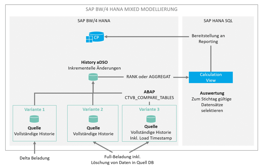
Our scenario works a little differently. While loading the source aDSO, we want to generate a timestamp for each data record that we load. This "load timestamp" shows us the validity date of the data record for the data model in SAP BW. This makes analysis easier later on in BW operation. Generating a load timestamp means that the changelog can no longer generate a delta. When loading our history aDSO, it can sometimes be difficult to filter out the new, changed, or deleted records from this source. New and changed records can only be determined manually using complicated table comparisons. The standard function module (FuBa) CTVB_COMPARE_TABLES provides a remedy.
CALL FUNCTION 'CTVB_COMPARE_TABLES'
  EXPORTING
    table_old        = lt_old
    table_new        = lt_new
    key_length       = lv_key
*   IF_SORTED        =
 IMPORTING
   TABLE_DEL        = lt_del
   TABLE_ADD        = lt_add
   TABLE_MOD        = lt_mod
*  NO_CHANGES       = .
FuBa compares two internal tables of the same type and returns new, changed, and deleted records in three corresponding internal tables:
- TABLE_DEL with all deleted records,
- TABLE_ADD with all new records, and
- TABLE_MOD with all changed records.
The key length (key_length) of the table to be compared is specified in bytes.
To use the function module, the data to be compared from the source (full data source) and target (with incremental history) must be prepared accordingly.
This is particularly necessary for the existing history: While the full data source already contains all the data to be compared, the status valid on the load date must first be determined from the history. In the above example of incremental history, key A with quantity 20, which was loaded on January 2, is still valid on January 4, as no subsequent changes or deletions have been made.
The data status on January 4 is therefore as follows. Key B is no longer relevant as it has been marked for deletion:
Older records (e.g., A from January 1, 2020) are not selected because a newer record for A already exists. The selection can be made, for example, by a loop through the history (sorted by load date), in which only the key combinations with the most recent load date are processed. All changes are determined via the subsequent function module call. The three internal tables can then be added to the history with a new load date, whereby deleted records are still marked with a deletion indicator.
Assuming that the full load on January 5, 2020, looks as follows:
| Date (Key 1) | Key 2 | quantity |
|---|---|---|
| 05.01.2020 | A | 10 |
| 05.01.2020 | D | 10 |
Compared to the previous day, quantity A has changed and quantity C has been deleted. The full load is compared with the history from January 4, 2020:
| Date (Key 1) | Key 2 | quantity |
|---|---|---|
| 02.01.2020 | A | 20 |
| 03.01.2020 | C | 5 |
Then the internal tables returned by the function module each have one entry and look as follows:
| table | Key | quantity |
|---|---|---|
| TABLE_MOD | A | 10 |
| TABLE_DEL | C | 5 |
| TABLE_ADD | D | 10 |
All three tables are added to the history with a new load date, so the final history looks like this:
| Date (Key 1) | Key 2 | quantity | deletion flag | |
|---|---|---|---|---|
| 01.01.2020 | A | 10 | ||
| 01.01.2020 | B | 15 | ||
| 02.01.2020 | A | 20 | ||
| 03.01.2020 | C | 5 | ||
| 04.01.2020 | B | 0 | X | |
| 05.01.2020 | A | 10 | Change entry A | |
| 05.01.2020 | C | 0 | X | Delete entry C |
| 05.01.2020 | D | 10 | New entry D |
The advantage of this approach is that the history grows much more slowly than would be the case with complete snapshots. It is also independent of the load date. The history can run at any interval (even during the day) and always shows the status valid on the load date.
In order to report the data in a meaningful way (after all, a filter based on the load date would only contain the changes loaded on that day, but not the history that was valid at that time), there are two options available via Calculation View, which are presented below.
Reporting on incremental history via calculation view
If you want to report on an incremental history, it is not sufficient to filter by the load date. This would only capture the records that were changed on the load date. For complete reporting, all key combinations must be read with the current load date.
As an example, here is a history with changes over 5 days:
As of January 5, 2020, the following rates must be read:
| 05.01.2020 | A | 10 |
| 05.01.2020 | D | 10 |
As of January 3, however, the following rates would apply, including those that were already loaded on January 1 and 2, since no subsequent load with the same key took place:
| 01.01.2020 | B | 15 |
| 02.01.2020 | A | 20 |
| 03.01.2020 | C | 5 |
This behavior can be implemented very easily using a calculation view. There are two approaches available: the RANK function and the AGGREGATION function.
RANK functions
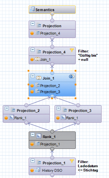
The basic idea behind using the rank function is to sort the source data in descending order by its load date using its keys and to insert a rank column: The highest rank of a key combination reflects the most recent load of this combination, while the lowest rank reflects the oldest load.
The data generated in this way is written in two projections:
1. Unchanged, including rank
2. New calculated column with column rank – 1
When the projections created in this way are joined via key and rank, each record is assigned a second load date, namely that of the subsequent load. The result is effectively a validity period for the respective key combination. Since the current record of a key combination has no successor, its "valid until" field is empty or zero.
| From (Key 1) Projection 2 | Until (Key 2) Projection 3 | Key 3 | quantity | deletion flag |
|---|---|---|---|---|
| 01.01.2020 | 01.01.2020 | A | 10 | |
| 01.01.2020 | 03.01.2020 | B | 15 | |
| 02.01.2020 | 04.01.2020 | A | 20 | |
| 03.01.2020 | 04.01.2020 | C | 5 | |
| 04.01.2020 | empty | B | 0 | X |
| 05.01.2020 | empty | A | 10 | |
| 05.01.2020 | empty | C | 0 | X |
| 05.01.2020 | empty | D | 10 |
Durch Filterung auf diesen Nullwert in der neuen „gültig bis“-Spalte können alle zum Stichtag gültigen Daten abgefragt werden. Durch Filterung der Quelldaten auf Ladedatum <= Stichtag, welcher per Parameter etwa bis in eine BW Query durchgereicht werden kann, kann der Snapshot jedes beliebigen Stichtages ermittelt werden.
RANK setting in Projection
Complete calculation view
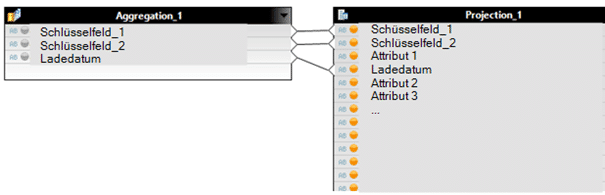
aggregation function
Durch eine Aggregation über alle Schlüsselfelder einer inkrementellen Historie und die Nutzung der Engine Aggregation MAX auf dem Ladedatum, lassen sich die jeweils zu einem Stichtag gültigen Schlüsselkombinationen + Ladedatum ermitteln. Damit das für beliebige Stichtage funktioniert, müssen die Quelldaten zunächst gefiltert werden: Ladedatum <= Stichtag. Dieser Filter kann per Parameter bis in eine BW Query durchgereicht werden.
Since aggregation only takes place on the key fields, all remaining fields must then be added again via a join. Since the aggregation provides the exact key, this is not a problem.
AGGREGATION: Load date with Enginge Aggregation MAX

Join the aggregation with complete history DSO:
Complete calculation view:

Comparison of RANK and AGGREGATION functions
Even though both calculation views deliver the same result, the choice between the RANK or AGGREGATION function is a question of the size of the history, the frequency of loading, and the reporting performance.
Example scenario: A history with 6 million key combinations grows to 60 million data records within a year. Since the RANK function assigns a rank to the entire history and joins it with itself, the calculation view must process a join of two tables with 60 million entries to obtain the current view of the data.
This is different with the AGGREGATION function: Aggregation first determines the currently valid keys (those with the current load date), which number only 6 million. For reporting purposes, these 6 million records are then joined with the complete history, i.e., 6 and 60 million. This join is much faster than it would be with two tables of equal size, each containing 60 million entries.
As the history grows, the use of the RANK function becomes increasingly slower, as more and more data has to be joined. The aggregation function, on the other hand, remains constant, as at least one of the two tables does not grow significantly. The allocated memory is also significantly smaller for aggregation.
The following screenshots show examples of how quickly the calculation views are executed when the history has grown from 6 to 60 million records after one year. In one case, the current data was retrieved, and in the other, the oldest data (valid one year ago) was retrieved:
RANK with current data (= reference date today, join of 60 and 60 million records)
AGGREGATION with current data (= today's key date, join of 60 and 60 million records)
RANK with one-year-old data (= reference date one year ago, join of 60 and 60 million records)
AGGREGATION with one-year-old data (= reference date one year ago, join of 60 and 60 million records)
Conclusion
For a long time, histories in SAP BW were backed up by creating snapshots. This tried-and-tested method continues to work well, but depending on the data model to be backed up and the frequency of the backup, the amount of data increases significantly over time. With SAP HANA-based systems, data redundancy should be avoided wherever possible – if only for cost reasons. Mixed modeling approaches offer new, more elegant ways to back up histories and query them efficiently. This minimizes the growth in data volume. Our example also shows how important it is for SAP BW developers to be familiar with both worlds (SAP BW + HANA SQL). The combination of the two is where the particular strength of hybrid data models lies.

Christopher Kampmann
Head of Business Unit
Data & Analytics
christopher.kampmann@isr.de
+49 (0) 151 422 05 448